Warp Drive Control Simulator — New Theory & Equations
Updated framework featuring Hawking–Ellis energy conditions, QEI bounds, sub-C synchronization, and +E/−E pairing for curvature control.
Live Demo: Warp Drive Engine (GitHub Pages)
Note: Theory & simulation only. Not engineering advice or operational guidance.
Purpose
This page consolidates the newest equations and control assumptions used in the Casanova warp framework. The simulator demonstrates how time-centric control can gate curvature strength, speed, and safety, while remaining consistent with known constraints (energy conditions, QEI bounds) in a theory-only context.
Foundations (concise)
- Einstein Field Equations (EFE): Gμν + Λ gμν = (8πG/c⁴) Tμν
- Stress-energy conservation: ∇μ Tμν = 0
- Alcubierre metric (warp bubble): ds² = -c²dt² + [dx - vs f(rs) dt]² + dy² + dz²
- Natário flow (zero expansion): shift-vector shaping for stability margins
- Hawking–Ellis energy conditions: WEC, SEC, NEC — enforced as throttling proxies in sim
- QEI bounds: negative energy localization bound by sampling time kernels
Velocity & Gradient Law
v = c · S · (warp)n · gf, with gradient factor
gf = √( ∫ |∇Φ|² dV / max_allowable )
- S: technology scale factor; n: warp exponent (fit to safety limits)
- Auto-throttle if gtt ≤ 0 (horizon risk) or proxy EC violation
Sub-C Synchronization (CST-Lock)
- Universal Magnetic Frequency drive: oscillatory fields near Earth Schumann (~7.83 Hz) for timing cadence
- Casanova Synchronized Time (CST) keeps onboard time phase-locked to Earth rhythms
- Constant-g travel (flip profile) with relativistic kinematics:
d = (c²/a)[cosh(a t / c) − 1], v(t) = (a t)/√(1+(a t / c)²)
+E / −E Pairing & QEI Compliance (theory)
Intent: Satisfy Hawking–Ellis constraints statistically while using localized negative-energy pulses that respect Quantum Energy Inequality (QEI) bounds.
- Paired energy channels: route −E micro-pulses (Casimir-scaled metamaterials) with time-symmetric +E in a high-Q superconducting loop; target recycling efficiency η ≥ 0.9999.
- Representative QEI bound: ∫⟨Tμνu^μu^ν⟩ f(τ)² dτ ≥ −K/τ₀⁴ (sampling function f of width τ₀).
- Balanced curvature nozzle: Cartesian-form Alcubierre shaping with matched +/− curvature rims to keep interior Minkowski-flat: ds² ≈ −c²dt² + dx² + dy² + dz².
Clock-Driven Control (C1–C5)
- C1: CSTClock (Earth anchor)
- C2: planetClock (destination rotation/orbit)
- C3: ibtClock (Interstellar Beacon Time)
- C4: ugtClock (Universal Galactic Time)
- C5: qClock (ns-grade quantum sync)
J = Σ w_i (T_Ci − T_C1)² → coilCurrents = Kp·ΔT + Kd·ΔṪ + Ki·∫ΔT dt
ΔT = ship time − CST. Residual timing error is mapped to coil shaping (rim steepness σ, effective radius R, pulse phase).
Trajectory & Motion (sim v3.6.x)
Curve: quadratic Bezier Earth→target with warp-dependent flattening
γ(u) = (1−u)² P0 + 2(1−u)u C + u² P1, u∈[0,1]
- curveHeight = C_base · [1 − warp/10] (Warp 1 high arc → Warp 10 nearly straight)
- Jerk-limited profile; arrival glow at u→1; clocks freeze on arrival
- ETA uses path length ∥γ′(u)∥ and speed cap from EC/QEI proxies
Relativistic Visuals
- Aberration: cosθ′ = (cosθ − β)/(1 − β cosθ)
- Doppler: λ′/λ = √((1+β)/(1−β))
Safety Proxies
- Horizon risk: gtt ≤ 0 → throttle
- Tidal/jerk bounds → widen rim, slow ramps
- Energy budget cap from reactor power → curvature ceiling
Materials (today)
- REBCO/Nb₃Sn coils & high-Q resonators
- Pulsed confinement & MW-class modulators
- Metamaterial tiles for −E localization (theory)
What’s New on This Page
- Explicit Hawking–Ellis (WEC/SEC/NEC) proxy gating in the control law
- QEI-aware +E/−E pairing model with recycling efficiency target
- Sub-C synchronization equations (cosh/sinh constant-g travel)
- Clear throttle rules for gtt, tidal, and jerk limits
- Refined gradient factor gf coupling to warp exponent n
Run the Demo & Read More
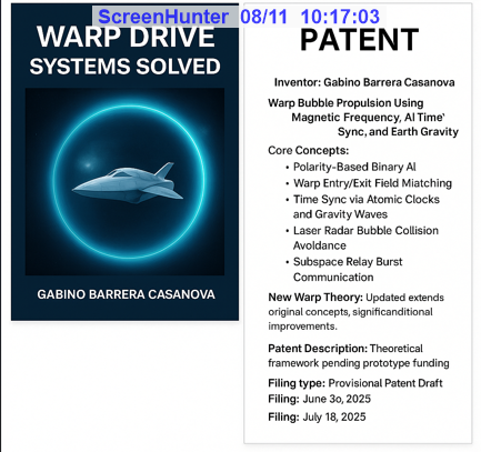
Patent Pending: Provisional filings dated 06/30/2025 and 07/15/2025. This page is an authorship and IP notice. The content is theoretical; do not attempt construction or operation of any device based on these ideas.